Measuring Performance with PStats

QUICK INTRODUCTION

PStats is Panda’s built-in performance analysis tool. It can graph frame rate over time, and can further graph the work spent within each frame into user-defined subdivisions of the frame (for instance, app, cull and draw), and thus can be an invaluable tool in identifying performance bottlenecks. It can also show frame-based data that reflects any arbitrary quantity other than time intervals, for instance, texture memory in use or number of vertices drawn.

The performance graphs may be drawn on the same computer that is running the Panda client, or they may be drawn on another computer on the same LAN, which is useful for analyzing fullscreen applications. The remote computer need not be running the same operating system as the client computer.

To use PStats, you first need to run the PStats server program, which is part of the Panda3D installation on Windows and Linux. On macOS, it is not included, but it can be built from source if the GTK+ 2 library is available on the system.

Once it is running, launch your application with the following set in your Config.prc file:

want-pstats 1

Or, at runtime, issue the Python command:

PStatClient.connect()

Or if you’re running pview, press shift-S.

Any of the above will contact your running PStats server program, which will proceed to open a window and start a running graph of your client’s performance.

If you have multiple computers available for development, it can be advantageous to run the pstats server on a separate computer so that the processing time needed to maintain and update the pstats user interface isn’t taken from the program you are profiling. If you wish to run the server on a different machine than the client, start the server on the profiling machine and add the following variable to your client’s Config.prc file, naming the hostname or IP address of the profiling machine:

pstats-host profiling-machine-ip-or-hostname

Profiling Python Code

If you are developing Python code, you may be interested in reporting the relative time spent within each Python task (by subdividing the total time spent in Python, as reported under “Show Code”). To do this, add the following line to your Config.prc file before you start ShowBase:

pstats-tasks 1

As of Panda3D 1.10.13 and Python 3.6 or higher, it is also possible to get a more detailed view of which specific Python modules, classes and functions are taking up time in the application. Note that this may slow down your application somewhat due to the fact that information is collected each time a function is called. To enable this, add the following line:

pstats-python-profiler 1

To access this view, in the Frame strip chart, double-click the App collector on the left side, then double-click the Python collector. Then, you can drill down further into the packages, modules, classes and functions.

Profiling GPU Time

OpenGL is asynchronous, which means that function calls aren’t guaranteed to execute right away. This can make performance analysis of OpenGL operations difficult, as the graphs may not accurately reflect the actual time that the GPU spends doing a certain operation. However, if you wish to more accurately track down rendering bottlenecks, you may set the following configuration variable:

pstats-gpu-timing 1

This will enable a new set of graphs that use timer queries to measure how much time each task is actually taking on the GPU.

Note

Please make sure you are at least using Panda3D 1.10.12 when trying to use this feature. Older versions had a bug that made GPU timing not work correctly with some graphics cards.

If your card does not support it or does not give reliable timer query information, a crude way of working around this and getting more accurate timing breakdown, you can set this:

gl-finish 1

Setting this option forces Panda to call glFinish() after every major graphics operation, which blocks until all graphics commands sent to the graphics processor have finished executing. This is likely to slow down rendering performance substantially, but it will make PStats graphs more accurately reflect where the graphics bottlenecks are.

THE PSTATS SERVER (The user interface)

The GUI for managing the graphs and drilling down to view more detail is entirely controlled by the PStats server program. At the time of this writing, there are two different versions of the PStats server, one for Unix and one for Windows, both called simply pstats. The interfaces are similar but not identical; the following paragraphs describe the Windows version.

When you run pstats.exe, it adds a program to the taskbar but does not immediately open a window. The program name is typically “PStats 5185”, showing the default PStats TCP port number of 5185; see “HOW IT WORKS” below for more details about the TCP communication system. For the most part you don’t need to worry about the port number, as long as server and client agree (and the port is not already being used by another application).

Each time a client connects to the PStats server, a new monitor window is created. This monitor window owns all of the graphs that you create to view the performance data from that particular connection. Initially, a strip chart showing the frame time of the main thread is created by default; you can create additional graphs by selecting from the Graphs pulldown menu.

Time-based Strip Charts

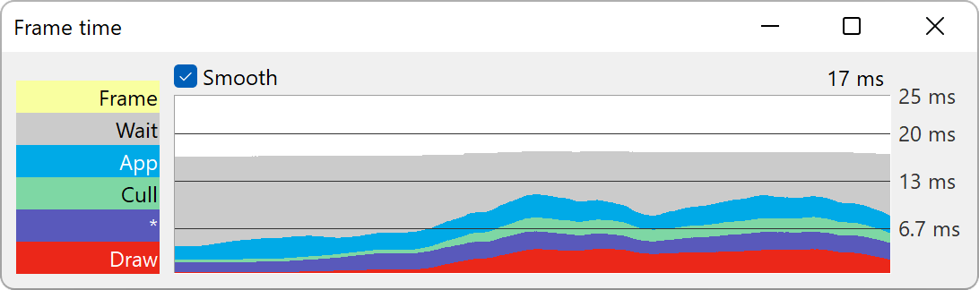
This is the graph type you will use most frequently to examine performance data. The horizontal axis represents the passage of time; each frame is represented as a vertical slice on the graph. The overall height of the colored bands represents the total amount of time spent on each frame; within the frame, the time is further divided into the primary subdivisions represented by different color bands (and labeled on the left). These subdivisions are called “collectors” in the PStats terminology, since they represent time collected by different tasks.

Normally, the three primary collectors are App, Cull, and Draw, the three stages of the graphics pipeline. Atop these three colored collectors is the label “Frame”, which represents any remaining time spent in the frame that was not specifically allocated to one of the three child collectors (normally, there should not be significant time reported here).

The frame time in milliseconds, averaged over the past three seconds, is drawn above the upper right corner of the graph. The labels on the guide bars on the right are also shown in milliseconds; if you prefer to think about a target frame rate rather than an elapsed time in milliseconds, you may find it useful to select “Hz” from the Units pulldown menu, which changes the time units accordingly. As of Panda3D 1.10.13, a counter may also be shown in the top-right corner keeping track of how many times during a frame the collector is started.

The running Panda client suggests its target frame rate, as well as the initial vertical scale of the graph (that is, the height of the colored bars). You can change the scale freely by clicking within the graph itself and dragging the mouse up or down as necessary. One of the horizontal guide bars is drawn in a lighter shade of gray; this one represents the actual target frame rate suggested by the client. The other, darker, guide bars are drawn automatically at harmonic subdivisions of the target frame rate. You can change the target frame rate with the Config.prc variable pstats-target-frame-rate on the client.

You can also create any number of user-defined guide bars by dragging them into the graph from the gray space immediately above or below the graph. These are drawn in a dashed blue line. It is sometimes useful to place one of these to mark a performance level so it may be compared to future values (or to alternate configurations).

The primary collectors labeled on the left might themselves be further subdivided, if the data is provided by the client. For instance, App is often divided into Show Code, Animation, and Collisions, where Show Code is the time spent executing any Python code, Animation is the time used to compute any animated characters, and Collisions is the time spent in the collision traverser(s).

To see any of these further breakdowns, double-click on the corresponding colored label (or on the colored band within the graph itself). This narrows the focus of the strip chart from the overall frame to just the selected collector, which has two advantages. Firstly, it may be easier to observe the behavior of one particular collector when it is drawn alone (as opposed to being stacked on top of some other color bars), and the time in the upper-right corner will now reflect just the total time spent within just this collector. Secondly, if there are further breakdowns to this collector, they will now be shown as further colored bars. As in the Frame chart, the topmost label is the name of the parent collector, and any time shown in this color represents time allocated to the parent collector that is not accounted for by any of the child collectors.

You can further drill down by double-clicking on any of the new labels; or double-click on the top label, or the white part of the graph, to return back up to the previous level.

Value-based Strip Charts

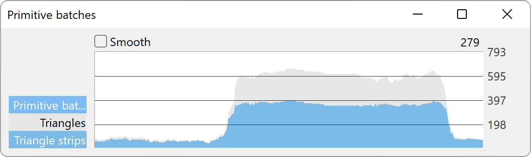
There are other strip charts you may create, which show arbitrary kinds of data per frame other than elapsed time. These can only be accessed from the Graphs pulldown menu, and include things such as texture memory in use and vertices drawn. They behave similarly to the time-based strip charts described above.

Piano Roll Charts

This graph is used less frequently, but when it is needed it is a valuable tool to reveal exactly how the time is spent within a frame. The PStats server automatically collects together all the time spent within each collector and shows it as a single total, but in reality it may not all have been spent in one continuous block of time.

For instance, when Panda draws each display region in single-threaded mode, it performs a cull traversal followed by a draw traversal for each display region. Thus, if your Panda client includes multiple display regions, it will alternate its time spent culling and drawing as it processes each of them. The strip chart, however, reports only the total cull time and draw time spent.

Sometimes you really need to know the sequence of events in the frame, not just the total time spent in each collector. The piano roll chart shows this kind of data. It is so named because it is similar to the paper music roll for an old- style player piano, with holes punched down the roll for each note that is to be played. The longer the hole, the longer the piano key is held down. (Think of the chart as rotated 90 degrees from an actual piano roll. A player piano roll plays from bottom to top; the piano roll chart reads from left to right.)

Unlike a strip chart, a piano roll chart does not show trends; the chart shows only the current frame’s data. The horizontal axis shows time within the frame, and the individual collectors are stacked up in an arbitrary ordering along the vertical axis.

The time spent within the frame is drawn from left to right; at any given time, the collector(s) that are active will be drawn with a horizontal bar. You can observe the CPU behavior within a frame by reading the graph from left to right. You may find it useful to select “pause” from the Speed pulldown menu to freeze the graph on just one frame while you read it.

Note that the piano roll chart shows time spent within the frame on the horizontal axis, instead of the vertical axis, as it is on the strip charts. Thus, the guide bars on the piano roll chart are vertical lines instead of horizontal lines, and they may be dragged in from the left or the right sides (instead of from the top or bottom, as on the strip charts). Apart from this detail, these are the same guide bars that appear on the strip charts.

The piano roll chart may be created from the Graphs pulldown menu.

Additional threads

If the panda client has multiple threads that generate PStats data, the PStats server can open up graphs for these threads as well. Each separate thread is considered unrelated to the main thread, and may have the same or an independent frame rate. Each separate thread will be given its own pulldown menu to create graphs associated with that thread; these auxiliary thread menus will appear on the menu bar following the Graphs menu.

Color and Other Optional Collector Properties

If you do not specify a color for a particular collector, it will be assigned a random color at runtime. At present, the only way to specify a color is to modify panda/src/pstatclient/pStatProperties.cxx, and add a line to the table for your new collector(s). You can also define additional properties here such as a suggested initial scale for the graph and, for non-time-based collectors, a unit name and/or scale factor. The order in which these collectors are listed in this table is also relevant; they will appear in the same order on the graphs. The first column should be set to 1 for your new collectors unless you wish them to be disabled by default. You must recompile the client (but not the server) to reflect changes to this table.

HOW TO DEFINE YOUR OWN COLLECTORS

The PStats client code is designed to be generic enough to allow users to define their own collectors to time any arbitrary blocks of code (or record additional non-time-based data), from either the C++ or the Python level.

The general idea is to create a PStatCollector for each separate block of code you wish to time. The name which is passed to the PStatCollector constructor is a unique identifier: all collectors that share the same name are deemed to be the same collector.

Furthermore, the collector’s name can be used to define the hierarchical relationship of each collector with other existing collectors. To do this, prefix the collector’s name with the name of its parent(s), followed by a colon separator. For instance, PStatCollector("Draw:Flip") defines a collector named “Flip”, which is a child of the “Draw” collector, defined elsewhere.

You can also define a collector as a child of another collector by giving the parent collector explicitly followed by the name of the child collector alone, which is handy for dynamically-defined collectors. For instance, PStatCollector(draw, "Flip") defines the same collector named above, assuming that draw is the result of the PStatCollector("Draw") constructor.

Once you have a collector, simply bracket the region of code you wish to time with collector.start() and collector.stop(). It is important to ensure that each call to start() is matched by exactly one call to stop(). If you are programming in C++, it is highly recommended that you use the PStatTimer class to make these calls automatically, which guarantees the correct pairing; the PStatTimer’s constructor calls start() and its destructor calls stop(), so you may simply define a PStatTimer object at the beginning of the block of code you wish to time. If you are programming in Python, you must call start() and stop() explicitly.

When you call start() and there was another collector already started, that previous collector is paused until you call the matching stop() (at which time the previous collector is resumed). That is, time is accumulated only towards the collector indicated by the innermost start() .. stop() pair.

Time accumulated towards any collector is also counted towards that collector’s parent, as defined in the collector’s constructor (described above).

It is important to understand the difference between collectors nested implicitly by runtime start/stop invocations, and the static hierarchy implicit in the collector definition. Time is accumulated in parent collectors according to the statically-defined parents of the innermost active collector only, without regard to the runtime stack of paused collectors.

For example, suppose you are in the middle of processing the “Draw” task and have therefore called start() on the “Draw” collector. While in the middle of processing this block of code, you call a function that has its own collector called “Cull:Sort”. As soon as you start the new collector, you have paused the “Draw” collector and are now accumulating time in the “Cull:Sort” collector. Once this new collector stops, you will automatically return to accumulating time in the “Draw” collector. The time spent within the nested “Cull:Sort” collector will be counted towards the “Cull” total time, not the “Draw” total time.

If you wish to collect the time data for functions, a simple decorator pattern can be used below, as below:

from panda3d.core import PStatCollector
def pstat(func):
    collectorName = "Debug:%s" % func.__name__
    if hasattr(base, 'custom_collectors'):
        if collectorName in base.custom_collectors.keys():
            pstat = base.custom_collectors[collectorName]
        else:
            base.custom_collectors[collectorName] = PStatCollector(collectorName)
            pstat = base.custom_collectors[collectorName]
    else:
        base.custom_collectors = {}
        base.custom_collectors[collectorName] = PStatCollector(collectorName)
        pstat = base.custom_collectors[collectorName]
    def doPstat(*args, **kargs):
        pstat.start()
        returned = func(*args, **kargs)
        pstat.stop()
        return returned
    doPstat.__name__ = func.__name__
    doPstat.__dict__ = func.__dict__
    doPstat.__doc__ = func.__doc__
    return doPstat

To use it, either save the function to a file and import it into the script you wish to debug. Then use it as a decorator on the function you wish to time. A collection named Debug will appear in the Pstats server with the function as its child.

from pstat_debug import pstat

@pstat
def myLongRunFunction():
    """ This function does something long """

HOW IT WORKS (What’s actually happening)

The PStats code is divided into two main parts: the client code and the server code.

The PStats Client

The client code is in panda/src/pstatclient, and is available to run in every Panda client unless it is compiled out. (It will be compiled out if OPTIMIZE is set to level 4, unless DO_PSTATS is also explicitly set to non-empty.)

The client code is designed for minimal runtime overhead when it is compiled in but not enabled (that is, when the client is not in contact with a PStats server), as well as when it is enabled (when the client is in contact with a PStats server). It is also designed for zero runtime overhead when it is compiled out.

There is one global PStatClient class object, which manages all of the communications on the client side. Each PStatCollector is simply an index into an array stored within the PStatClient object, although the interface is intended to hide this detail from the programmer.

Initially, before the PStatClient has established a connection, calls to start() and stop() simply return immediately.

When you call PStatClient.connect(), the client attempts to contact the PStatServer via a TCP connection to the hostname and port named in the pstats- host and pstats-port Config.prc variables, respectively. (The default hostname and port are localhost and 5185.) You can also pass in a specific hostname and/or port to the connect() call. Upon successful connection and handshake with the server, the PStatClient sends a list of the available collectors, along with their names, colors, and hierarchical relationships, on the TCP channel.

Once connected, each call to start() and stop() adds a collector number and timestamp to an array maintained by the PStatClient. At the end of each frame, the PStatClient boils this array into a datagram for shipping to the server. Each start() and stop() event requires 6 bytes; if the resulting datagram will fit within a UDP packet (1K bytes, or about 84 start/stop pairs), it is sent via UDP; otherwise, it is sent on the TCP channel. (Some fraction of the packets that are eligible for UDP, from 0% to 100%, may be sent via TCP instead; you can specify this with the pstats-tcp-ratio Config.prc variable.)

Also, to prevent flooding the network and/or overwhelming the PStats server, only so many frames of data will be sent per second. This parameter is controlled by the pstats-max-rate Config.prc variable and is set to 30 by default. (If the packets are larger than 1K, the max transmission rate is also automatically reduced further in proportion.) If the frame rate is higher than this limit, some frames will simply not be transmitted. The server is designed to cope with missing frames and will assume missing frames are similar to their neighbors.

The server does all the work of analyzing the data after that. The client’s next job is simply to clear its array and prepare itself for the next frame.

The PStats Server

The generic server code is in pandatool/src/pstatserver, and the GUI-specific server code is in pandatool/src/gtk-stats and pandatool/src/win-stats, for Unix and Windows, respectively. (There is also an OS-independent text-stats subdirectory, which builds a trivial PStats server that presents a scrolling- text interface. This is mainly useful as a proof of technology rather than as a usable tool.)

The GUI-specific code is the part that manages the interaction with the user via the creation of windows and the handling of mouse input, etc.; most of the real work of interpreting the data is done in the generic code in the pstatserver directory.

The PStatServer owns all of the connections, and uses network sockets to communicate with the clients. It listens on the specified port for new connections, using the pstats-port Config.prc variable to determine the port number (this is the same variable that specifies the port to the client). Usually you can leave this at its default value of 5185, but there may be some cases in which that port is already in use on a particular machine (for instance, maybe someone else is running another PStats server on another display of the same machine).

Once a connection is received, it creates a PStatMonitor class (this class is specialized for each of the different GUI variants) that handles all the data for this particular connection. In the case of the windows pstats.exe program, each new monitor instance is represented by a new toplevel window. Multiple monitors can be active at once.

The work of digesting the data from the client is performed by the PStatView class, which analyzes the pattern of start and stop timestamps, along with the relationship data of the various collectors, and boils it down into a list of the amount of time spent in each collector per frame.

Finally, a PStatStripChart or PStatPianoRoll class object defines the actual graph output of colored lines and bars; the generic versions of these include virtual functions to do the actual drawing (the GUI specializations of these redefine these methods to make the appropriate calls).